Domain adaptation with Xception and VGG16 models

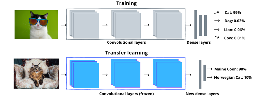
When beginning a journey with artificial intelligence algorithms, it is worth asking yourself two fundamental questions:

1. What is the issue we are trying to solve?
2. How to build a model that will assist in solving this issue?

To answer the first question, the only limiting factors are our imagination and the availability of data we can use for training the model. And for the second question, which model to choose will largely depend on the following: the problem we are solving, available resources and the time frame we have at our disposal.

This is best shown on an example. Let’s assume that we are trying to create an algorithm that helps segregate waste properly based on a photo. When it comes to selecting the algorithm itself, it will depend on the posed problem. We could use random decision forests or support vector machines after we extract the appropriate features from the image. We could also use convolutional neural networks, which operate directly on the image data. We can design the architecture of this network ourselves. It is worth, however, to consider a pre-trained model, which will allow for saving a lot of time. To solve this problem I have decided to adopt pre-trained artificial neural networks for image classification. How does this look in practice? Let’s go through the process step by step.

Data analysis and preparation

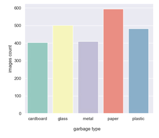
The data set that I decided to use can be found  here: Garbage Classification. It contains photos of waste divided into 6 categories: cardboard, glass, metal, paper, plastic and mixed waste. The last category contains photos of items that could largely be assigned to the other 5 groups. For this reason, we exclude it from further analysis. Below is a graph showing the number of photos available for each class.

A very important stage in the preparation of the data set is  to divide it into at least two subsets:  the training and validation subsets. An even better practice is to create three separate sets of data: training, validation and test. In this case, the results obtained on the test set are representative and show the real effectiveness of the system for new, previously unseen photos. In my case, 60% of the photos were used for training, 20% was a validation set, and another 20% went to the test set.

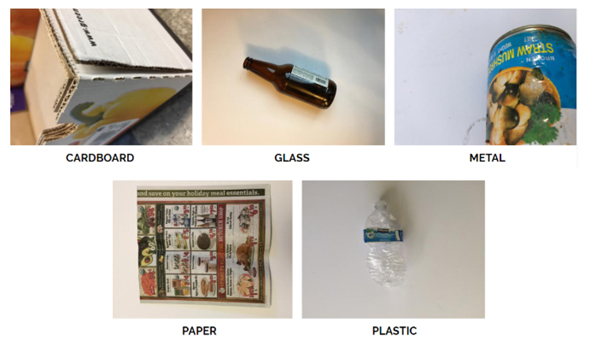
Below are sample photos for each class. Each photo is 512 x 384 pixels. When using a ready neural network, it is very important to adjust the size of the images in the set to the size of the input data accepted by the network. In the case of the Xception network, the size of the input layer is 299 x 299, while in the case of the VGG16 network, this size is 224 x 224. Therefore, before training the model, we need to scale our images.

Preparation and training of models

To solve the given problem, I used two popular network architectures: VGG16 and Xception. Both models I selected were pre-trained on the ImageNet collection, which contains pictures of objects belonging to 1000 classes. Therefore, the output layer responsible for the classification of the input image has 1000 outputs. In the case of the problem we are analyzing, the size of the output layer should be 5. Below is the code that allows for adapting the pre-trained model to our data set.

# model adaptation
21   base_net=tf.keras.applications.xception.Xception(weights='imagenet')
22   base_net_input  = base_net.get_layer(index=0).input
23   base_net_output = base_net.get_layer(index=-2).output
24   base_net_model  = models.Model(inputs=base_net_input, outputs=base_net_output)
25   
26   for layer in base_net_model.layers:
27      layer.trainable = False
28   
29   new_xception_model = models.Sequential()
30   new_xception_model.add(base_net_model)
31   new_xception_model.add(layers.Dense(5, activation='softmax', input_dim=2048))

Due to the limited data set used for training the model, I decided to expand it using data augmentation. Below is a fragment of the code responsible for training the selected model.

# hyperparameters
34   base_learning_rate = 0.0001
35   opt = optimizers.SGD(lr=1e-3, decay=1e-6, momentum=0.9, nesterov=True)
36   
37   new_xception_model.compile(optimizer=opt,
38                loss='sparse_categorical_crossentropy',
39                metrics=['accuracy'])
40   
41   # data preparation and augmentation
42   train_datagen = ImageDataGenerator(
43          rescale=1./255,
44          shear_range=0.2,
45          zoom_range=0.2,
46          horizontal_flip=True)
47   
48   valid_datagen = ImageDataGenerator(rescale=1./255)
49   
50   train_generator = train_datagen.flow_from_directory(
51      directory='training_data',
52      target_size=img_dim,
53      color_mode="rgb",
54      batch_size=batch_size,
55      class_mode="sparse",
56      shuffle=True,
57      seed=42
58   )
59   
60   valid_generator = valid_datagen.flow_from_directory(
61      directory='validation_data',
62      target_size=img_dim,
63      color_mode="rgb",
64      batch_size=batch_size,
65      class_mode="sparse",
66      shuffle=True,
67      seed=42
68   )
69   
70   # model training
71   garbage_recognition_model = new_xception_model.fit_generator(generator=train_generator,
72                      validation_data=valid_generator,
73                      epochs=epochs,
74                      callbacks=[checkpoint, tensorboard_callback, earlyStop]
75   )

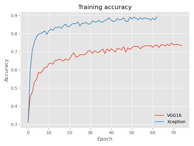
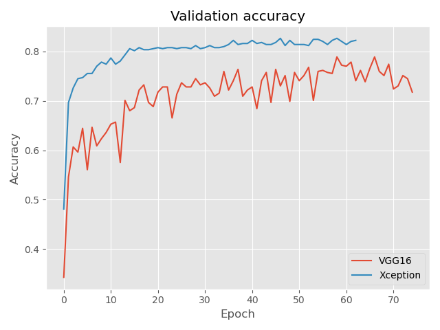
During the training of selected models I used early stopping. The way it works is that if the recognition efficiency of photos from the validation set does not increase over a certain number of epochs, training is interrupted. Using this type of approach reduces the risk of the model overfitting to the data. Below are the learning curves for the training and validation sets. It is evident that in this case the Xception network did much better, achieving more than 80% efficiency in recognizing photos from the validation set.

Effectiveness of the created solutions

As I mentioned beforehand, it is best to determine the actual effectiveness of our model on a new data set that did not participate in training of our models. Therefore, below I present the results that were achieved by letting the models tackle the test set. This collection contained 480 photos. The results confirm the conclusion that in this case the model based on the pre-trained Xception network did much better. It achieved an efficiency of 83%, which is almost 10 percentage points more than the model based on the VGG16 architecture.

VGG16

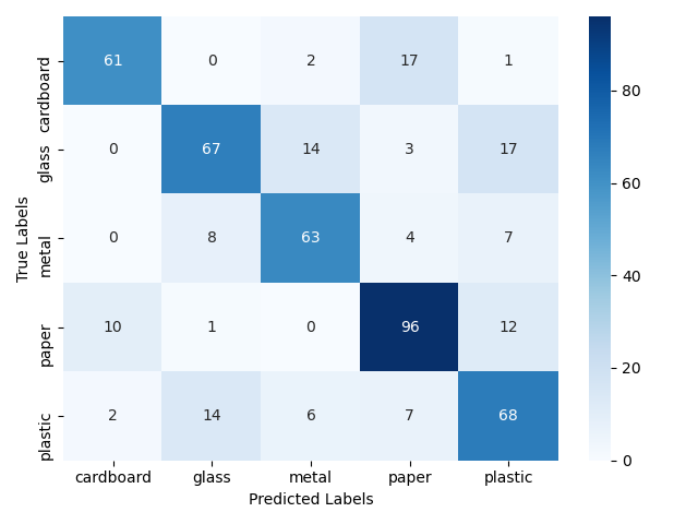
ACC = 74%

Xception

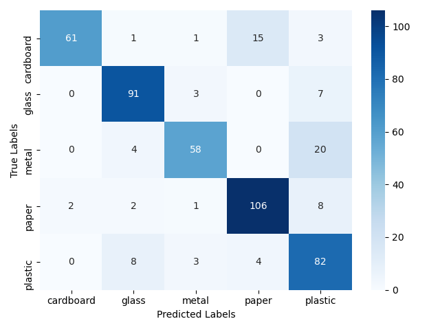
ACC = 83%

Summary

The article shows how to use pre-trained network architectures and apply them to a specific problem that we want to solve. The process of data analysis and preparation, adaptation of pre-trained models to one’s needs and methods of assessing the effectiveness of the created solution are briefly discussed.

This is the first in a series of articles intended for people who want to start their adventure artificial intelligence algorithms. I invite you to follow our entries on the Isolution blog and our company profiles on LI and FB, as well as to subscribe to our newsletter.